The Data Importer Object
This object imports data from an external file in comma-separated value (CSV) format and uses it to create particles. For a full discussion of the way this works and some examples of its use, please see the page 'Importing/Exporting Particle Data'.
If you are not familiar with the use of this object please read the above overview page before using it for the first time.
Interface
This is the object's interface:
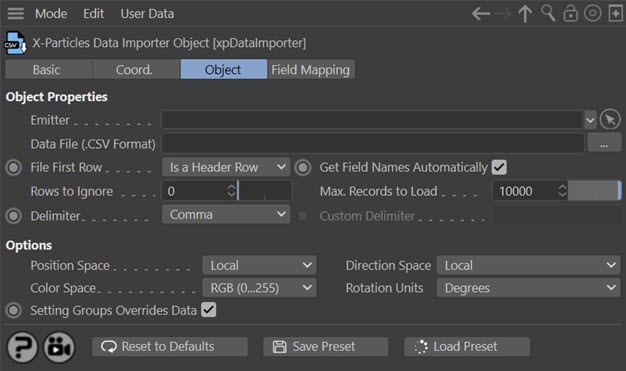
For the buttons at the bottom of the interface, please see the 'Common interface elements' page.
The Field Mapping tab is discussed lower down this page.
Parameters
Emitter
Drag an emitter into this field. This is the emitter which will be used to create the new particles.
The emitter will automatically be switched into 'Controlled Only' mode. It is recommended that you do NOT alter this. Also, the emitter speed will be set to zero. You can change this but if you do, the new particles will be created and then the emitter will move them with the speed given in the emitter. This will result in the position being offset slightly from that specified in the source data file.
Important: any emitter used in a data importer CAN NOT be cached. This is a limitation due to the way the system works.
Data File
This is the data file which will provide the source data from which to create particles. It must be in CSV format (see the page 'Importing/Exporting Particle Data' for details).
File First Row
This is a very important setting and you may need to open the data file in a text editor or spreadsheet to check if there is a header row. If there is a header row, it should be the first line in the file and will contain a list of field names rather than numeric values. See 'Importing/Exporting Particle Data' for details of the CSV file header row.
There are two options in this drop-down menu:
Is a Header Row
With this option, the first line in the file is assumed to be a header row.
Is a Data Row
In this case it is assumed that the file has no header row and that the first line must be actual data.
What happens if you get this wrong? There are three possibilities.
The file has a header row but you select 'Is a Data Row'
If you do this, the importer will create a set of standard field names, which will be Field1, Field2, etc. You will then have to use these names when mapping the data fields to particle data rather than the names in the header. In addition, the importer will assume the first row is actual data, so will try to convert a series of text strings into numbers...which is unlikely to work, so the values for that first line will all be zeros.
The file does not have a header row but you select 'Is a Header Row'
In this case the importer will take the first row (which is actually data) and convert it into text for use as the field names. If the first field has a value of -98.34, the first field name will be "-98.34" (without the apostrophes) and you will have to use that name to map the field to particle data. Also, you will lose the first line of data as it will be used as the field names instead.
The file may or may not have a header row but the first line(s) in the file are neither a header nor data
This happens if the file author inserted some comment lines at the start of the file. If you have such a file, you need to count how many such lines there are and instruct the importer to ignore them using the 'Rows to Ignore' setting. The importer will then treat the first line after the ignored rows as either a data row or a header row, depending on the setting in 'File First Row'.
Get Field Names Automatically
If this switch is checked, whenever the data file changes the importer will scan the file and build a list of field names, using the settings in 'File First Row' and 'Rows to Ignore'. This list will then be available to you as a drop-down list when adding field maps. If the switch is unchecked no field list will be built and you will have to enter the field names manually.
It is strongly recommended that you leave this switch checked and only uncheck it if you really need to (e.g. if faced with an unusual file format from which the field names cannot be obtained).
Rows to Ignore
A correctly-formatted CSV file should only contain an optional header row plus the data rows themselves. However, some files have one or more lines of text at the start, before the header/data rows. In this case you can either remove them with a text editor, or use this setting.
If you specify a number greater than zero in this setting the importer will ignore that many rows at the start of the file. So if, for example, you set this to 2, the importer will ignore the first two lines and the first row (as far as the importer is concerned) is actually the third line in the file. That line could be either a header row or a data row, of course.
Max. Records to Load
Some data files can be huge. If you only want to use a subset of the data, set this value to however many rows of data you want to use.
Delimiter
This drop-down lets you indicate which character is used as a delimiter in the data file. The most common is a comma, but tabs and semicolons are also popular. Use the drop-down to specify the delimiter to use. If you have a file which uses something else, you can select 'Other' then enter the character in the 'Custom Delimiter' field.
Custom Delimiter
This is the field delimiter character to use if 'Other' is selected in the 'Delimiter' setting.
Caution: you should only enter one character! If you enter a string of two or more characters the data importer will try to use that, and it will work - as long as the data file uses a string rather than a single character. If it doesn't, the data import will fail.
Options
These are additional options that you can change depending on the data file being used.
Position Space
When position data for the new particle is imported it can be treated as either 'World' or 'Local' data. This drop-down lets you select which one to use.
If you choose 'World' the data is treated as being in 3D world space, so no matter where the emitter is located the particle will be created at that point in 3D space. If 'Local' is selected, the position is taken as relative to the emitter, so the actual position in the 3D world will vary, depending on the emitter position. The default is 'Local'.
Direction Space
This is exactly the same as the 'Position Space' setting except that the imported particle direction is either set to 'World' or 'Local' space. The default is 'Local'.
Color Space
Colour values in data files may take several different formats and this drop-down lets you choose which one to use. You will almost certainly need to open the file in a text editor or spreadsheet to find out which format is used, unless the author of the file has provided that information. The possible options are:
RGB (0...255)
This is probably the commonest choice. The colour is expressed in three data fields, one for red, green, and blue respectively. A value of 0 means there is none of that component in the final colour, a value of 255 means that component is at its maximum amount.
RGB (0...1)
Exactly the same as RGB (0...255) except that the range is given from 0.0 to 1.0. (This is the format used internally by X-Particles.)
RGB (0...100%)
Exactly the same as RGB (0...1) except that the range is given from 0.0% to 100.0%.
HSV
The colour is in Hue, Saturation and Value format.
HSL
The colour is in Hue, Saturation and Luminance format.
Color Index
This is a special mode used by astronomers to represent star colours. Unlike all the other options, this is a single value rather than three separate ones.
Important: if this method is used, the color index in the data file MUST be mapped to the 'Color: Red' data field (see 'Field Mapping' below).
Rotation Units
If the data file contains rotation values, these can be expressed in either degrees or radians. Select the method used from this drop-down.
Setting Groups Overrides Data
This switch is only relevant if you want the imported data to set the particle group. If it is checked, and you have mapped data in the data file to the group number, the parameters of that group (colour, etc.) will override the corresponding imported data values. Normally you would probably want that to happen so this switch is checked by default. Unchecking it will cause the group number to be set in the particle but no other changes will be made.
See the section 'Setting groups from imported data' below for more information.
Field Mapping
Important note: Before you start adding field maps, ensure that you have specified a data file and set the above options as required. The reason is that changing certain options will automatically cause all the field maps to be reset (i.e. deleted). This is because changing them will alter the data structure the importer expects and to ensure that you don't get a mismatch between the maps and the file, all maps are removed.
The options which, if changed, will reset the maps are:
- the data file itself
- the file first row setting
- the switch to get the field names automatically
- the number of rows to ignore
- the delimiter, or the custom delimiter if 'Delimiter' is set to 'Other'
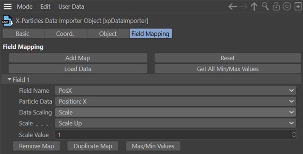
Once the various options have been set, you can now map the fields in the data file to specific items of particle data. This is done in the field mapping tab:
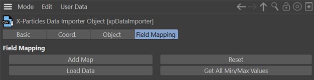
Initially this is empty because no maps have been set up yet.
Note that you don't have to map every data field in the file to something in the particle. In fact, in many cases you won't be able to, because there is no equivalent item of particle data. That doesn't matter; you can safely ignore any fields you don't want or can't use.
Add Map
To add a map, click the large 'Add Map' button. You will need one map for each field in the data you want to map (so position data, for example, will need three maps - one each for the X, Y, and Z coordinates). You don't need to add maps in the same order as the fields in the data file; any order is fine.
Reset
Clicking this button will delete all your field maps. You will be asked to confirm this before the maps are deleted.
Load Data
Clicking the 'Load Data' button will cause the data to be loaded and mapped. Note that you MUST reload the data by clicking this button every time you make changes to the field maps, since the mapped data is stored in memory and must be refreshed if changes have been made.
(You don't need to reload the data if you add or remove maps, just if you change any of the values in an existing map.)
Get All Min/Max Values
If you click this button, the importer will scan the loaded data and will calculate the minimum and maximum values for each data item, then insert these values into the 'Data Range Min.' and 'Data Range Max.' fields. These are used when squashing (range mapping) the data; see below for more details.
Because this will alter all the ranges in one go, you are asked to confirm that you want to do this. If you only need the minimum and maximum values to be calculated for one or two data items, you can use the 'Max/Min Values' button in the individual maps.
Don't forget to click 'Load Data' again after using this button or the new ranges will not be used!
Setting map parameters
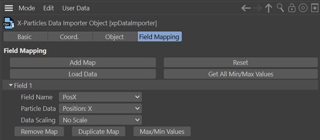
Once you have added a map you can set the parameters. There are only two you must enter: the field name and the data item it maps to. The rest are optional. Assuming you have specified a data file, and that 'Get Field Names Automatically' is checked, the initial interface will look something like this (the field names will be different of course):
If you have not yet specified a data file, or if 'Get Field Names Automatically' was turned off, you will see this:
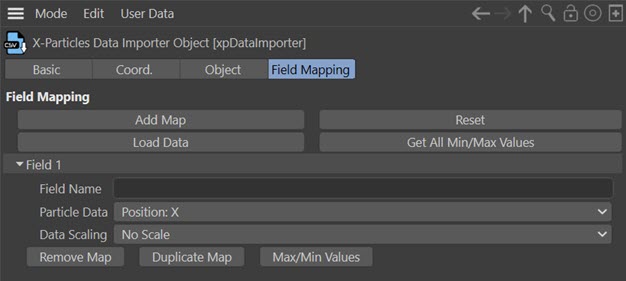
The difference is that in the first instance you will have to enter the field name by hand into the 'Field Name' edit field, but in the second the field names are available for you in a drop-down menu. This is clearly much more convenient so it is recommended that before adding maps you specify the data file and leave 'Get Field Names Automatically' turned on.
Field Name
Either select the required field from the drop-down list or type the name of the field to map in this box. The name is the name of the field that comes from the header row in the CSV file (if it has one - if it didn't have a header row, the fields are all named 'Field1', 'Field2', 'Field3', etc, in order across the row).
Particle Data
From this drop-down menu you select the item of particle data to map this field to. Note that position, direction, rotation and in most cases colour, are three individual fields. The possible data items to map to are shown in this table:
| Data Item | Comment |
| Position: X | The X-coordinate of the particle position |
| Position: Y | The Y-coordinate of the particle position |
| Position: Z | The Z-coordinate of the particle position |
| Direction: X | The X-coordinate of the particle direction vector (see note 1 below) |
| Direction: Y | The Y-coordinate of the particle direction vector (see note 1 below) |
| Direction: Z | The Z-coordinate of the particle direction vector (see note 1 below) |
| Speed | The particle's speed (but see note 1 below) |
| Radius | The particle's radius in scene units |
| Group Number | An integer which corresponds to one of the particle groups in the scene (see note 2 below) |
| Age | The particle's age in seconds |
| Lifespan | The particle's lifespan in seconds |
| Color: Red | The red component of the particle's colour (when using one of the RGB colour modes - see note 3 below) |
| Color: Blue | The blue component of the particle's colour (when using one of the RGB colour modes - see note 3 below) |
| Color: Green | The green component of the particle's colour (when using one of the RGB colour modes - see note 3 below) |
| Rotation: H | The H component of the particle's rotation (see note 4 below) |
| Rotation: P | The P component of the particle's rotation (see note 4 below) |
| Rotation: B | The B component of the particle's rotation (see note 4 below) |
| Mass | The particle's mass |
| Temperature | The particle's temperature |
| Smoke | The particle's smoke value |
| Fuel | The particle's fuel value |
| Fire | The particle's fire value |
Notes
- X-Particles expects the particle direction to be in the form of a normalised direction vector, not Euler angles.
- The group number must be the number of one of the particle groups in the scene. See the section 'Setting groups from imported data' below for more information.
- In the RGB colour modes these three field are always named 'Color: Red' etc. In HSV mode they will change to 'Hue', 'Saturation', and 'Value' instead; in HSL mode, they will read 'Hue', 'Saturation', and 'Luminance'. If the mode is 'Color Index' the 'Color: Red' field will become 'Color Index' and the other two fields are ignored.
- Although rotations will be imported, to have any effect you must turn on rotations in the emitter, otherwise you will not see any rotation occurring even though the data is loaded.
Make sure you map the field to the correct item of particle data! If you don't you will either get no particles at all, or they will be in the wrong position, etc.
Data Scaling
For the reason why this parameter is necessary, please see the section 'The problem of scaling data' below.
This drop-down controls how the imported data will be scaled to produce the correct results. It has three options:
No Scale
The imported data will be used as is, and will not be scaled in any way.
Scale
The imported data will be scaled up or down by a simple numeric factor. Select whether you want to scale up or down from the 'Scale' setting and enter the scale factor in the 'Scale Value' box. In this mode the interface changes to look like this:
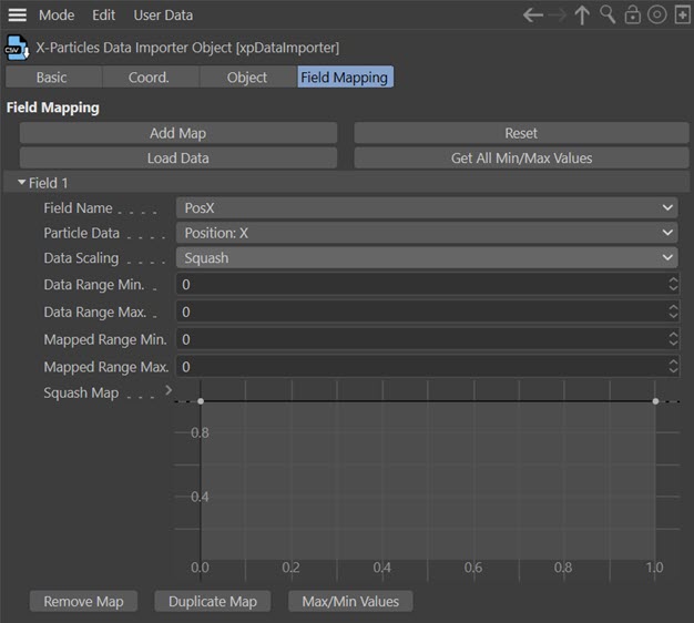
Squash
The imported data will be squashed into a different range. This is discussed more fully below. The interface will appear like this:
Don't forget to click 'Load Data' again after changing this setting or the new scale will not be used!
Scale
A simple drop-down with two entries:
Scale Up
The data value will be scaled up by the value in 'Scale Value'.
Scale Down
The data value will be scaled down by the value in 'Scale Value'.
Don't forget to click 'Load Data' again after changing this setting or the new scale will not be used!
Scale Value
The scale factor to use in 'Scale' mode. Note that a value of zero will cause the data value always to be zero as well.
Data Range Min., Data Range Max.
These are the limits of the data range to map in 'Squash' mode. They can be whatever you like but normally you would set 'Data Range Min.' to the lowest value in the data field and 'Data Range Max.' to the largest value. But you can change these ranges if you like. For example, suppose the lowest value is 1 and the highest is 100. In most cases you would use these two values for the minimum and maximum. But you could set them to 10 and 90 if you wished; then the data fields with values 1 to 10 would all have the same value and the data fields with values 90 to 100 would also have a common value.
Note: the minimum value cannot be larger than the maximum value. They can be the same value but if the minimum value is the larger of the two the range will be set to zero.
Mapped Range Min., Mapped Range Max.
These are the upper and lower limits of the values the data fields will be mapped to in 'Squash' mode. They can be whatever you like. You can even set them to be outside the 'Data Range Min.' and 'Data Range Max.' values if you wish - this will cause the range of values to be stretched rather than squashed!
Note: as with the data range values, the minimum value cannot be larger than the maximum value. They can be the same value but if the minimum value is the larger of the two the range will be set to zero. Among other things, this means you cannot map a data range of 0 to 100 to a mapped range of 0 to -100. You can, however, map a data range of 0 to 100 to a mapped range of -100 to 0.
Squash Map
This spline is used to control the distribution of values. In many cases you can ignore this spline control, but it may be useful for some data. See the next section for details of how it is used.
Note that in the default setting this spline has no effect and the data is controlled entirely by the data and mapped value ranges.
Remove Map
Click this button to remove the map.
Duplicate Map
If you click this button the map is duplicated and added to the end of the list of maps. This is often quicker than clicking 'Add Map' and is particularly useful if you need to copy the 'Squash Map' spline from another map.
Min/Max Values
Clicking this button will cause the data importer to scan all the values for this particular data item (e.g. particle speed) and insert them into the 'Data Range Min.' and 'Data Range Max.' fields. This is a lot easier than scanning through tens of thousands of lines of data trying to work out the data range you need!
Don't forget to click 'Load Data' again after using any of the above settings or the new ranges will not be used!
The problem of scaling data
Let us suppose that you have a data file with a field named 'Size' and you want to map this to the particle radius. The range of values in 'Size' is from 1 to 100, which means that if you use the data without scaling it, you will have particles whose radius may be as small as 1 scene unit, and some with a radius of up to 100 scene units - which is huge (for particles!).
How you deal with this is what the scaling mode is for. The simplest way is to choose 'Scale' mode, select 'Scale Down' and enter a value of (say) 20. Now the radius will range from 5 (100 / 20 = 5) down to 0.05 (1 / 20 = 0.05). This may be fine but the problem is that a radius of 0.05 may be too small to be seen when rendered.
Ideally you would like that range of 1 to 100 to be something more reasonable - say 0.5 to 5. This is what 'Squash' mode is for. In this mode we are squashing a large range into a smaller one. Here's what you would do:
Set the data ranges
Set the 'Data Range Min.' and 'Data Range Max' parameters to the minimum and maximum values for that data item in the file. They don't have to be the exact values, any reasonable minimum and maximum values will do. Just remember that any data value at or below the 'Data Range Min.' value will be assigned the value in 'Mapped Range Min.' and the converse with the maximum values. Remember that you can use the 'Min/Max Values' button for any data item to set these ranges automatically, or the 'Get All Min/Max Values' button to get the data ranges for all data items.
In the above example you would set the minimum value to 1 and the maximum value to 100.
Don't forget to click 'Load Data' again after changing the data ranges or the new ranges will not be used!
Set the mapped ranges
These are the values the data will be mapped to. In the example you would set the mapped minimum value to 0.5 and the maximum to 5. All the data values will be mapped to this range, so that (for example) a data value halfway between the minimum and maximum will be mapped to a value halfway between the mapped minimum and maximum values.
Don't forget to click 'Load Data' again after changing the data ranges or the new ranges will not be used!
Adjust the Squash Map spline (optional)
The spline gives you finer control over the result. Suppose in the original example the data values were spread evenly between the values of 1 and 100. The mapped values will then be spread evenly between the values 0.5 and 5.
But suppose you really want the distribution of the values to be skewed towards the smaller end of the range? You can use the spline for this. If you adjust the spline like this:
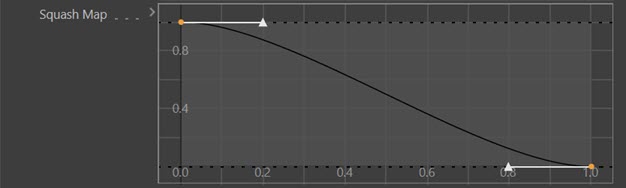
In this case the larger values will be scaled down. You will then see a cutoff for the value which will always be less than 5.
In most cases you will never need the spline control. But it is available if you do.
Don't forget to click 'Load Data' again after changing the spline or the new spline will not be used!
Setting groups from imported data
It is possible to specify the group the particle will be put in when it is created. To do this map a field in the data file to the 'Group Number' parameter in the particle data. The value in the file MUST be greater than zero; group zero is the default group used by the emitter when no other groups are used and this cannot be overridden. If a group with the specified number does not exist, the default emitter parameters will be used.
Mapping a data item to a group number will NOT cause a new group to be created. The group must already exist in the scene.
By default any settings in the group will override those in the imported data, so if the data contained a colour, this will be overridden by the group colour. However, the group mode will be used to determine which settings are overridden. If the mode is set to 'Display Only' only the colour and colour mode will be overridden; if the imported data set other values such as mass or radius, these will not be changed. However, if the group mode is set to 'Standard' the imported speed will be overridden; mass would only be overridden if the group mode was set to 'Extended'.
You can prevent all of the imported data from being overridden by unchecking the 'Setting Groups Overrides Data' switch in the options section. Then the only thing which is changed is the group number.
Emitter and group
Normally for a particle to be emitted belonging to a specific group that group must be in the 'Groups to Use' list of the emitter. (It can be changed later, of course.) With the data importer the group does not have to be in the 'Groups to Use' list of the emitter to use the group parameters, UNLESS the group colour mode is set to 'Gradient (Parameter)'. For this to work correctly the emitter must be able to access the group, so if you want the imported particles to use that mode in the assigned group, be sure to drag the group into the emitter's 'Groups to Use' list.
Execution speed
Finally, you should be aware that assigning the particle to a group and setting the group colour mode to any of the gradient or shader modes will result in a slower load process. This will probably only be noticeable with large numbers of imported particles.